Rise of the Phillips Curve Theories of job search were developed in large part to understand the Phillips curve. The Phillips curve was based on a 1958 article by A.W. Phillips in which he noted that there was a relationship between unemployment rates and changes in wage rates in the United Kingdom. Economists saw his results as a missing piece to the Keynesian multiplier model, and after a slight alteration (changing the wage rates to prices), his curve became one of the most famous curves in economics. The graph below shows the combinations of unemployment and inflation that the United States experienced in the 1950s and 1960s. Each point represents one year and tells the rate of inflation and unemployment for that year. For example, in 1953 the rate of inflation was 1.6% and the rate of unemployment was 2.9%. This year is represented by one of the two points off the line closest to the origin. Notice how the points tend to cluster around a downward-sloping curve. This curve is the Phillips curve. 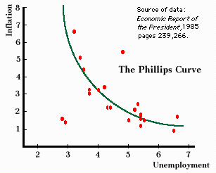The Phillips curve became important when economists began to interpret it as a curve showing the range of possibilities open to the economy. This interpretation was perhaps natural given the tendency for economists to think in terms of tradeoffs. Economists believe that free lunches are very rare; that to get something desirable, one almost always must give up something. The Phillips curve seemed to be a trade-off: to get reduced unemployment, the economy must suffer from more inflation, and to get reduced inflation, the economy must suffer from more unemployment. The Phillips curve completed the Keynesian multiplier model, which before 1960 contained only real or constant-price values and did not claim to explain prices. The Phillips curve opened a way for this model to add the rate of inflation as a variable it could predict. The model would explain real output, and each level of real output could be associated with an unemployment rate. With the Phillips curve each level of unemployment could be associated with a rate of inflation. The major problem for policy makers then became one of trying to balance the benefits of more employment against the costs of higher inflation. Once they had decided which point on the Phillips curve was best, they believed that they could use fiscal and monetary policy to attain it. Some economists had enough faith in their understanding of how the economy worked that they began to talk about abolishing recessions forever and of "fine tuning" the economy. The addition of the Phillips curve changed the aggregate supply and aggregate demand curves implied in the Keynesian multiplier model. The model no longer had to assume the horizontal aggregate supply curve. It now had an upward-sloping supply curve (but with rates of inflation, not price level, on the vertical axis). One can get from the Phillips curve to an upward sloping curve by putting employment rate rather than unemployment rate on the axis. Although the aggregate demand curve remained vertical, the resulting model was a far more attractive theory than one that could say nothing about inflation, a key variable of macroeconomics. Economic results in the 1960s seemed to confirm the interpretation of the Phillips curve as a long-run and stable trade-off. As the decade passed, the U.S. economy got lower and lower unemployment rates and higher and higher rates of inflation. The idea of the unemployment-inflation trade-off became part of the conventional wisdom and even began appearing in principles textbooks. But the 1970s were to challenge this neat and tidy picture. Copyright Robert Schenk